Aritifical neural networks seem chaotic but in actuality are very structured. Shoutout to NN SVG for the image.

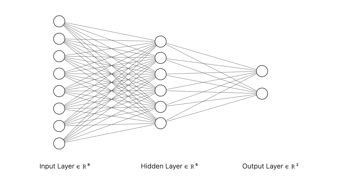
You do not need to be an expert on ANNs to understand that their is a clear and ordered flow to the network. Inputs go through the input layer, and ouputs come from the output layer.

There are various kind of ANNs, some that have residual connections, some with convolutional layers, and some with more complex layers like transformers. The main point is, when it comes to feedforward NNs there seems to consistently be an idea of layers, where one layer feeds to another.

There exist a number of reasons why this layer to layer paradigm is followed (compute efficiency, generalizability, etc...), but for now, I want to forget all of those and reimagine the feedforward NN. Please note, the this is similar to something already well established called NEAT (neural evolution of augmenting topologies), though I have not seen it implimented as we do in this and the following article(s).

We are building what I call a Chaos Network. The name is probably already used for something else, but for now, we will use it to describe a feedforward neural network that does not use the standard layer to layer paradigm. Instead, think of it as an acyclic graph where nodes are semi-randomly connected to one another.

We will build this completely from scratch implimenting our own automatic differntiation library (a very simple one), and train the Chaos Network on MNIST to see how our network performs.

Spoiler, with our current version we achieve around 91% accuracy, not great (yet).

As we are building this from scratch, we must first craft the foudation of our Chaos Network: tensors and automatic differentiation. For those not familiar, the type of tensor we are referring to is one the machine learning community has coined, not the tensor as meant in mathematics. Basically all of the code in the following sections is highly inspired by dfdx, a "shape checked deep learning library". If you are not familiar with dfdx, but work in ML with Rust, I highly encourage you to check it out!

The type of reverse mode automatic differentiation we are implimenting relies heavily on the chain rule. We are essentially creating an abstraction around a Rusts's f32 type we call a tensor. This tensor has its own set of mathemetical methods we can perform on it, and something we call a tape. The tape records all mathematical operations the tensor is involved with, and then allows us to replay those operations using the chain rule, computing the gradients for the associated tensor.

We will break it down in parts. First let's examine the tensor definition.

#[derive(Debug)]
pub struct Tensor0D {
    pub id: i32,
    pub data: f32,
    pub tape: Option<Tape>,
}

The only thing of note not mentioned above is that we call it Tensor0D implying that there may be tensors of higher dimensions. Spoiler: in normal libraries there are, but in our simple one we stay in the first dimension.

Let's briefly look at the definition of the Tape and some of its associated functions.

#[derive(Default)]
pub struct Tape {
    operations: Vec<Box<dyn FnOnce(&mut Gradients)>>,
}

impl Tape {
    pub fn add_operation(&mut self, operation: Box<dyn FnOnce(&mut Gradients)>) {
        self.operations.push(operation)
    }

    pub fn merge(&mut self, mut other: Self) {
        other.operations.append(&mut self.operations);
        self.operations = other.operations;
    }

    pub fn execute(&mut self) -> Gradients {
        let mut gradients: Gradients = Gradients::default();
        for operation in self.operations.drain(..).rev() {
            (operation)(&mut gradients);
        }
        gradients
    }
}

Tape has an attribute called operations, that is a vector storing a series of closures taking in a Gradients struct. It has two associated functions that allow it to add operations and merge other tapes.

The most important piece to note is the associated function execute. In this function we are replaying the tape and passing in Gradients.

#[derive(Debug, Default)]
pub struct Gradients {
    grads: HashMap<i32, Tensor0D>,
}

impl Gradients {
    pub fn remove(&mut self, id: i32) -> Tensor0D {
        self.grads
            .remove(&id)
            .unwrap_or(Tensor0D::default_without_tape())
    }

    pub fn insert(&mut self, key: i32, tensor: Tensor0D) {
        self.grads.insert(key, tensor);
    }
}

The Gradients struct is almost as simple, storing a HashMap of <i32, Tensor0D>. The grads (HashMap) stores the gradients of the tensor with the associated id. It may be worth noting that if you view dfdx's implimentation, you would find that the HashMap and remove and insert associated functions would not use Tensor0D, but would use Box<dyn Any>. In our case the gradients are always a Tensor0D but if we supported tensors of other dimensions, it would be possilble to have gradients of Tensor1D or Tensor2D.

Let's look at an associated operation for the Tensor0D.

impl<'a, 'b> Mul<&'b mut Tensor0D> for &'a mut Tensor0D {
    type Output = Tensor0D;

    fn mul(self, other: &'b mut Tensor0D) -> Self::Output {
        let mut new = Tensor0D::new_without_tape(self.data * other.data);

        new.tape = match (self.tape.take(), other.tape.take()) {
            (Some(mut self_tape), Some(other_tape)) => {
                self_tape.merge(other_tape);
                let new_id = new.id;
                let self_id = self.id;
                let other_id = other.id;
                let self_data = self.data;
                let other_data = other.data;
                self_tape.add_operation(Box::new(move |g| {
                    let mut tg1 = g.remove(new_id);
                    let mut tg2 = tg1.clone();
                    tg1.data *= other_data;
                    tg2.data *= self_data;
                    g.insert(self_id, tg1);
                    g.insert(other_id, tg2);
                }));
                Some(self_tape)
            }
            (Some(mut self_tape), None) => {
                let new_id = new.id;
                let self_id = self.id;
                let other_data = other.data;
                self_tape.add_operation(Box::new(move |g| {
                    let mut tg = g.remove(new_id);
                    tg.data *= other_data;
                    g.insert(self_id, tg);
                }));
                Some(self_tape)
            }
            (None, Some(mut other_tape)) => {
                let new_id = new.id;
                let other_id = other.id;
                let self_data = other.data;
                other_tape.add_operation(Box::new(move |g| {
                    let mut tg = g.remove(new_id);
                    tg.data *= self_data;
                    g.insert(other_id, tg);
                }));
                Some(other_tape)
            }
            (None, None) => None,
        };

        new
    }
}

The above code allows us to run and assert the following test:

fn test_mul_0d() {
    let mut a = Tensor0D::new_with_tape(1.);
    let mut b = Tensor0D::new_with_tape(2.);
    let mut c = &mut a * &mut b;
    // Check value match
    assert_eq!(2., c.data);
    // Check gradients
    let mut grads = c.backward();
    let a_grads = grads.remove(a.id);
    let b_grads = grads.remove(b.id);
    assert_eq!(2., a_grads.data);
    assert_eq!(1., b_grads.data);
}

We have done it! We have very simple automatic differntiation. This test could be expanded to support any number of variations of variables multiplied together. It won't work for a few key scenarios where a or b are reused later. In that scenario, we would have to account for the law of total derivatives. This won't be an issue for us.

In addition to the mul associated funtion, we also impliment add, mish, and nll (negative log likelihood). I won't be showing these here, but they are available in the repo.

With the foundation of automatic differntiation done, we can move on to creating the actual network.

As our network is an acylic graph, we need a way to represent that graph.

#[derive(Default)]
pub struct Network {
    inputs: Vec<Rc<RefCell<Node>>>,
    pub nodes: Vec<Rc<RefCell<Node>>>,
    pub leaves: Vec<Rc<RefCell<Node>>>,
    mode: NetworkMode,
}

pub struct Node {
    id: i32,
    pub weights: Vec<Tensor0D>,
    connections: Vec<Rc<RefCell<Node>>>,
    running_value: Tensor0D,
    running_hits: i32,
    connected_from: i32,
    kind: NodeKind,
    leaf_id: i32,
}

Because we need to have shared references with mutability, we are using Rc and RefCell. This does introduce a small overhead, but I'm sure as you will see later, does not play a large part in hindering the performance of our network as there are much larger problems (thousands of function calls).

The Network holds Nodes in three vectors, inputs, nodes, and leaves. These three vectors are just for convenience and not all required.

The Node has an id, weights and connections, a running_value, running_hits, connected_from (the number of connections that are from different nodes to it), the kind (type of node), and the leaf_id (if it is a leaf). This implimentation of the leaf_id is lazy. There are better ways to do it.

Let's examine what it looks like to add a node to the network.

pub fn add_node(&mut self, kind: NodeKind) {
    let node = Node::new(kind);
    let node = Rc::new(RefCell::new(node));
    self.nodes.push(node.clone());
    match kind {
        NodeKind::Normal => {
            self.add_normal_node_first_connection(node.clone());
        }
        NodeKind::Input => {
            self.inputs.push(node.clone());
            for n in &self.leaves {
                (*node).borrow_mut().add_connection(n.clone());
            }
        }
        NodeKind::Leaf => {
            self.leaves.push(node.clone());
            for n in &self.inputs {
                (**n).borrow_mut().add_connection(node.clone());
            }
        }
    }
    for _i in 0..5 {
        self.connect_node(node.clone());
    }
}

The add_node function takes the kind of node as an argument, adds it the appropriate vector, and if it is an Input, or Leaf connects it to all of the leaves or inputs respectively. If it is a Normal node, it connects it between two already created nodes. At the end of the add_node function, we connect the newly added node with 5 other random nodes already in the network.

Here is where the name Chaos Network originated. Unlike the standard feedforward NNs, Chaos Network has no concept of layers, just nodes connected to one another in a random assortment.

The only other notable associated function for the Network is the forward function, all other functions are helpers around constructing the network and adding nodes.

pub fn forward(&mut self, mut input: Vec<Tensor0D>) -> Vec<Tensor0D> {
    let mut output: Vec<Tensor0D> = Vec::with_capacity(self.leaves.len());
    output.resize(self.leaves.len(), Tensor0D::new_without_tape(0.));
    for (_i, n) in self.inputs.iter().enumerate() {
        (**n).borrow_mut().forward(input.remove(0), &mut output);
    }
    output
}

The forward function is very simple. We initialize a vector of tensors we iterate over our input nodes passing in the values passed to the network. In the case of MNIST we will have 784 input nodes we call forward on.

fn forward(&mut self, mut input: Tensor0D, output: &mut Vec<Tensor0D>) {
    self.running_hits += 1;
    let mut x = &mut self.running_value + &mut input;
    // If we do not have all of our data yet, comeback later
    if self.running_hits < self.connected_from {
        self.running_value = x;
        return;
    }
    // If we are done, reset the middle values
    self.running_value = Tensor0D::new_without_tape(0.);
    self.running_hits = 0;
    // If we are a leaf, push the value, else call forward on our connections
    match &self.kind {
        NodeKind::Leaf => {
            output[self.leaf_id as usize] = x;
        }
        _ => {
            x = &mut x
                + &mut (&mut Tensor0D::new_without_tape(1.)
                    * self.weights.first_mut().unwrap());
            if matches!(self.kind, NodeKind::Normal) {
                x = Tensor0D::mish(&mut x);
            }
            for (i, n) in self.connections.iter().enumerate() {
                (**n)
                    .borrow_mut()
                    .forward(&mut self.weights[i + 1] * &mut x, output);
            }
        }
    };
}

The forward for the Node (above) is slightly more complicated. First we increment running_hits, then we sum the input with our running_value, and check if all nodes that are connected to it have been included in the running_value. If they have not we return. This may seem unintutive, but in a situation where each node may have many connections, we do not want to continue forward through the network until the total input has been sent to this node. If you examine how normal feedforward NNs work, this idea is the same, although potentially harder to interpret in code.

Once all inputs have reached the node and been summed into the running_value we reset the running_value and running_hits so the network is ready for the next pass. We then check the kind of node we are in. If we are a Leaf, we save our value in the output. If we are not a Leaf, we add our bias and continue.

After adding the bias, we check if we are not an Input. If we are not an Input, we apply our activation function. In this case, we have chosen to use the mish activation function.

Finally, we call forward on all other connected nodes multiplying by the weight associated with that connection.

That is our Chaos Network minus the training, which we add quickly with the following associated functions in the Network and Node.

impl Network {
    pub fn backward(&mut self, mut loss: Tensor0D) {
        let mut gradients = loss.backward();
        let mut visited = HashMap::new();
        for n in self.inputs.iter() {
            (**n)
                .borrow_mut()
                .apply_gradients(&mut gradients, &mut visited);
        }
    }
}


impl Node {
  fn apply_gradients(&mut self, gradients: &mut Gradients, visited: &mut HashMap<i32, bool>) {
        if *visited.get(&self.id).unwrap_or(&false) {
            return;
        }
        visited.insert(self.id, true);
        for w in self.weights.iter_mut() {
            let w_gradients = gradients.remove(w.id);
            w.data -= 0.0025 * w_gradients.data;
            w.reset_tape();
        }
        for n in &self.connections {
            (**n).borrow_mut().apply_gradients(gradients, visited);
        }
    }
}

Now it is done!

Having created our network, let's train it on MNIST.

fn main() {
    let mnist = Mnist::new("data/");
    let mut network = build_network();

    for i in 0..TRAINING_EPOCHS {
        for ii in 0..EXAMPLES_PER_EPOCH {
            // Prep data
            let input: Vec<Tensor0D> = mnist.train_data[ii]
                .iter()
                .map(|x| Tensor0D::new_without_tape(*x as f32 / 255.))
                .collect();
            let label = mnist.train_labels[ii] as usize;

            // Forward pass
            let output = network.forward(input);
            let loss = Tensor0D::nll(output, label);
            network.backward(loss);
        }
        // Do end of epoch validation
        network.set_mode(NetworkMode::Inference);
        let percent_correct = validate(&mut network, &mnist);
        network.set_mode(NetworkMode::Training);
        println!(
            "Epoch: {} val_percent: {}",
            i,
            percent_correct
        );
    }
}

I have ommited a few things above, but that loop trains the network!

How does it perform? Not great.

Epoch: 1 val_percent: 0.8905
Epoch: 2 val_percent: 0.8972
Epoch: 3 val_percent: 0.9009
Epoch: 4 val_percent: 0.9046
Epoch: 5 val_percent: 0.9058
Epoch: 6 val_percent: 0.9062
Epoch: 7 val_percent: 0.9081
Epoch: 8 val_percent: 0.9079
Epoch: 9 val_percent: 0.908
Epoch: 10 val_percent: 0.9087
Epoch: 11 val_percent: 0.9085
Epoch: 12 val_percent: 0.9097
Epoch: 13 val_percent: 0.9096
Epoch: 14 val_percent: 0.9095
Epoch: 15 val_percent: 0.9097
Epoch: 16 val_percent: 0.9093
Epoch: 17 val_percent: 0.9092
Epoch: 18 val_percent: 0.9094
Epoch: 19 val_percent: 0.9099
Epoch: 20 val_percent: 0.9098
Epoch: 21 val_percent: 0.9102
Epoch: 22 val_percent: 0.9102
Epoch: 23 val_percent: 0.9103
Epoch: 24 val_percent: 0.91
Epoch: 25 val_percent: 0.91
Epoch: 26 val_percent: 0.9111
Epoch: 27 val_percent: 0.9113
Epoch: 28 val_percent: 0.9115
Epoch: 29 val_percent: 0.9117
Epoch: 30 val_percent: 0.9112
Epoch: 31 val_percent: 0.9117
Epoch: 32 val_percent: 0.9113
Epoch: 33 val_percent: 0.9113
Epoch: 34 val_percent: 0.9115
Epoch: 35 val_percent: 0.9114
Epoch: 36 val_percent: 0.9118
Epoch: 37 val_percent: 0.9121
Epoch: 38 val_percent: 0.9119
Epoch: 39 val_percent: 0.9122
Epoch: 40 val_percent: 0.9121
Epoch: 41 val_percent: 0.9117
Epoch: 42 val_percent: 0.9118
Epoch: 43 val_percent: 0.912
Epoch: 44 val_percent: 0.9117
Epoch: 45 val_percent: 0.9119
Epoch: 46 val_percent: 0.9118
Epoch: 47 val_percent: 0.9118
Epoch: 48 val_percent: 0.9117
Epoch: 49 val_percent: 0.9121

Note the val_percent is the percent our network gets correct on 10,000 items of test data (data not included in the training data).

Considering that random guessing will get about 10% correct, 91% is way better than guessing, but about 9% below state of the art feedforward NNs.

There are a few reasons why I think our network performed poorly. One, we did not use any batches. Batches are pretty much essential for stable training, and during training we did not use any. This was done because our network does not support 1D tensors yet (although we probably stil could have done batches). Two, the real potential of the network is not being utilized. The main reason I wanted to design a network like this is because it can change and grow very easily. New connections can be formed randomly, connections can be dropped, nodes can be added in strange positions. While the network we created is chaotic, it is not the final iteration.

Chaos Network in its final form should be constantly morphing, evolving and changing as the problems it faces grow more difficult, but we will see that in part 2.

Thanks for reading!

the repo